Tutorial 7: Data-driven turbulent combustion modeling
Note
The complete code associated with this tutorial is available here.
Learner profile
This tutorial is aimed at a user who has a solid understanding of Computational Fluid Dynamics (CFD) for Combustion. A basic understanding of machine learning is not required.
The tutorial could also be beneficial for those who do not have strong competencies in CFD but know Data Science; in fact, apart from some computations to extract interesting quantities in reacting flows, the basic operations that we are going to perform on the data are based on filtering of 3D fields. In case the overall code is too overwhelming at once, make sure to try the previous tutorials in this documentation.
Dataset description
The dataset used in this example is a sub-domain of the DNS dataset presented in [14, 22]. The configuration corresponds to a turbulent lifted hydrogen jet flame issuing into a heated air coflow at atmospheric pressure. The DNS is designed to investigate flame stabilization mechanisms close to the autoignition limit.
A diluted fuel mixture composed of 65% H2 and 35% N2 (by volume) is injected from a central slot at an inlet temperature of 400 K. The jet is surrounded on both sides by coflowing air streams at 850 K. The jet width at the inlet is 2 mm and the corresponding jet Reynolds number is 8000. Turbulent inflow conditions are imposed by superimposing velocity fluctuations with an intensity of 10% of the bulk jet velocity, generated from an auxiliary homogeneous isotropic turbulence field and prescribed at the inlet using Taylor’s hypothesis.
The full DNS domain comprises \(2000 \times 1600 \times 400\) grid points (\(15H \times 20H \times 3H\)) with uniform spacing in the streamwise and spanwise directions and a stretched transverse grid. The simulation is performed using the Sandia DNS solver S3D with a detailed hydrogen–air mechanism consisting of nine species and twenty-one elementary reactions developed by Li et al. [23].
In this tutorial, only a spatial sub-domain of the original dataset is employed to reduce memory requirements and improve reproducibility, while retaining the key physical and chemical features of the lifted flame configuration.

Figure 1: Graphical representation of the DNS subset used in the present example
A priori validation methodology
Favre Filtered species transport equation
In the context of Large Eddy Simulation (LES), the transport equation for the Favre-filtered mass fraction of species \(k\) reads
where:
\(\tilde{Y}_k\) is the Favre-filtered mass fraction of species \(k\),
\(j^{\mathrm{sgs}}_{k,i}\) is the subgrid-scale diffusive flux of species \(k\),
\(\overline{\dot{\omega}}_k\) is the filtered chemical source term.
In this tutorial, we focus on the closure of the chemical source term \(\overline{\dot{\omega}}_k\), which represents one of the main challenges in turbulent combustion modeling.
A priori evaluation of chemical source terms
From Direct Numerical Simulation (DNS) data, chemical source terms can be computed directly using detailed chemistry (e.g. through Cantera). Since DNS resolves both transport and chemical processes down to the finest relevant scales, the resulting reaction rates naturally account for the full interaction between turbulence and chemistry.
In a priori analysis, these DNS-based reaction rates are considered as reference values.
In contrast, LES does not have access to this level of detail. Only filtered quantities—such as temperature, velocity, pressure, and species mass fractions—are available. To mimic the information accessible in LES, the DNS fields are therefore filtered explicitly.
Starting from these filtered fields, chemical source terms can be recomputed using the same detailed chemistry models. However, because the filtering operation removes small-scale fluctuations, the resulting reaction rates are generally less accurate than those obtained from the original DNS data. In particular, transport processes are no longer resolved down to the Kolmogorov scale, and the interaction between turbulence and chemistry is only partially captured.
The comparison between:
reaction rates computed from the original DNS fields, and
reaction rates recomputed from the filtered fields,
forms the basis of the a priori validation framework used to assess turbulence–chemistry interaction closures.
Step 1: DNS data processing
In this first step, we extract from the DNS dataset all the quantities required to perform an a priori analysis and to build a data-driven closure model. The goal is to construct, from the DNS data, both reference quantities and LES-like quantities obtained by explicit filtering.
Dataset loading and initialization
We begin by specifying the path to the DNS sub-domain and initializing a
Field3D object. If the dataset is not found locally,
it is automatically downloaded.
import os
import aPriori as ap
from aPriori.DNS import Field3D

directory = os.path.join('.', 'Lifted_H2_subdomain')

T_path = os.path.join(directory, 'data', 'T_K_id000.dat')
if not os.path.exists(T_path):
    ap.download(dataset='h2_lifted')

DNS_field = Field3D(directory)
At this stage, the DNS field contains all primitive variables (velocity, temperature, species mass fractions) resolved down to the smallest scales.
Compute reaction rates on the DNS grid
Using the detailed chemical mechanism associated with the dataset, we compute the chemical source terms directly on the DNS grid. These reaction rates naturally account for the full interaction between turbulence and chemistry and are therefore used as reference values in the a priori analysis.
DNS_field.compute_reaction_rates()
The heat release rate (HRR) is computed automatically as part of this operation.
Filtering the DNS field
To mimic the information available in Large Eddy Simulation (LES), the DNS field is explicitly Favre-filtered. In this example, a filter width of \(\Delta = 16\) grid points is used.
It is important to note that the filtering operation applies to all variables present in the data folder. Since the DNS reaction rates have already been computed, they are filtered as well, yielding the filtered reference source terms \(\overline{\dot{\omega}}^{DNS}\).
filter_size = 16
filtered_field = Field3D(DNS_field.filter_favre(filter_size))
Compute reaction rates on the filtered field
Starting from the LES-like filtered quantities (filtered temperature and species mass fractions), reaction rates are recomputed using the same detailed chemistry. These rates correspond to a Laminar Finite Rate (LFR) approximation evaluated on filtered fields.
filtered_field.compute_reaction_rates()
The discrepancy between DNS-filtered and LFR reaction rates highlights the impact of unresolved turbulence–chemistry interactions.
Compute additional variables of interest
To train a data-driven closure model, additional LES-scale quantities are required. These are quantities that are often needed for modeling sub-filter interactions. In this tutorial, we compute:
the strain-rate magnitude,
the residual dissipation rate (Smagorinsky model),
the residual kinetic energy,
chemical and mixing time scales.
These quantities characterize the local interaction between turbulence and chemistry and are commonly used in subgrid-scale modeling.
filtered_field.compute_strain_rate(save_tensor=False)
filtered_field.compute_residual_dissipation_rate(mode='Smag')
filtered_field.compute_residual_kinetic_energy()

filtered_field.compute_chemical_timescale(mode='SFR')
filtered_field.fuel = 'H2'
filtered_field.ox = 'O2'
filtered_field.compute_chemical_timescale(mode='Ch')
filtered_field.compute_mixing_timescale(mode='Kolmo')
At the end of this step, the filtered field contains both LES-resolved variables and reference subgrid-scale quantities, enabling the construction of data-driven closure models.
Step 2: Neural network training
Prerequisites
This chapter supposes that the reader is already familiar with Neural Networks (NNs) and knows how to code using Pytorch. In case you’re not familiar with these concepts, I strongly suggest you the following sources:
Steve Brunton’s book ‘Data Driven Engineering’.
This video series from 3blue1brown is an insightful and clear explanation.
Pytorch documentation and tutorials are a complete source for learning this library.
The exercise of the class of Data-Driven Engineering for the 1st year master’s students
at Université Libre de Bruxelles. This source is less detailed but can provide quick, straightforward source of information if you already have a basic understanding of the topic.
Overview
In this second step, a neural network is trained to model the correction factor \(\gamma\) that accounts for unresolved turbulence–chemistry interactions. The approach follows the same conceptual framework used in models such as EDC and PaSR, where the filtered chemical source term is written as
The term \(\dot{\omega}^{QLFR}_k\) represents the quasi-laminar finite rates (QLFR) and typically involves the integration of a reactor in time. Our approach will be based on the laminar finite rates (LFR)
Here, \(\dot{\omega}^{LFR}_k\) is the reaction rate of the \(k^th\) species directly computed from filtered quantities, and \(\gamma\) is a data-driven term which represents the cell reacting fracion predicted by the neural network. Our optimization problem can hence be reduced to the computation of the factor \(\gamma\) such that some quantities of interest related to the reaction rates are optimized with respect to the reference DNS data. In the next steps we will further highlight this point.
Data preprocessing for PyTorch
We construct the input feature matrix using quantities available at LES scale: temperature, strain-rate magnitude, and the slowest chemical time scale. The target output is the DNS heat release rate.
import torch
import torch.nn as nn
import torch.optim as optim
import numpy as np
import matplotlib.pyplot as plt
from sklearn.model_selection import train_test_split

# DATA PROCESSING
T      = filtered_field.T.reshape_column() # extract the valeue of Temperature from the filtered field and rehape it as a column vector
S      = filtered_field.S_LES.reshape_column()
Tau_c  = filtered_field.Tau_c_SFR.reshape_column()

HRR_LFR = filtered_field.HRR_LFR.reshape_column()
HRR_DNS = filtered_field.HRR_DNS.reshape_column()
The input variables are normalized and transformed before building the training matrix.
T      = (T-np.min(T))/(np.max(T)-np.min(T))
S      = np.log10(S)
S      = (S-np.min(S))/(np.max(S) - np.min(S))
Tau_c  = np.log10(Tau_c)
Tau_c  = (Tau_c-np.min(Tau_c)) / (np.max(Tau_c)-np.min(Tau_c))

# Build the training data matrix
X = np.hstack([T, S, Tau_c])
The dataset is then split into training and testing subsets and converted to PyTorch tensors.
# Divide between train and test data
X_train, X_test, HRR_LFR_train, HRR_LFR_test, HRR_DNS_train, HRR_DNS_test = train_test_split(
   X, HRR_LFR, HRR_DNS, test_size=0.9, random_state=42)

X_train = torch.tensor(X_train, dtype=torch.float32)
X_test  = torch.tensor(X_test,  dtype=torch.float32)
HRR_LFR_train = torch.tensor(HRR_LFR_train, dtype=torch.float32)
HRR_LFR_test  = torch.tensor(HRR_LFR_test,  dtype=torch.float32)
HRR_DNS_train = torch.tensor(HRR_DNS_train, dtype=torch.float32)
HRR_DNS_test  = torch.tensor(HRR_DNS_test,  dtype=torch.float32)
Neural network architecture
The neural network is implemented as a fully connected feed-forward model using PyTorch. The architecture consists of multiple hidden layers with ReLU activation functions.
# NN class definition
class NeuralNetwork(nn.Module):
   def __init__(self, input_size, hidden_size, output_size, num_layers):
      super(NeuralNetwork, self).__init__()
      self.layers = nn.ModuleList() # initialize the layers list as an empty list using nn.ModuleList()
      self.layers.append(nn.Linear(input_size, hidden_size)) # Add the first input layer. The layer takes as input <input_size> neurons and gets as output <hidden_size> neurons
      for _ in range(num_layers - 1):
            self.layers.append(nn.Linear(hidden_size, hidden_size)) # Add hidden layers
      self.layers.append(nn.Linear(hidden_size, output_size)) # add output layer

   def forward(self, x):    # Function to perform forward propagation
      for layer in self.layers[:-1]:
            x = torch.relu(layer(x))
      x = self.layers[-1](x)
      return x

# NN architecture
input_size = 3
num_layers = 6
hidden_size = 64
output_size = 1
model = NeuralNetwork(input_size, hidden_size, output_size, num_layers)
Training loop
The neural network is trained by minimizing the mean squared error (MSE) between the DNS heat release rate and the corrected Laminar Finite Rate (LFR) prediction
The loss function and optimizer are first defined:
The optimizer acts on model.parameters(), which contains all learnable
weights and biases of the neural network layers. During training, these
parameters are iteratively updated to minimize the loss function.
To accelerate training, the model and tensors are transferred to the appropriate computational device. On Apple Silicon machines, the Metal Performance Shaders (MPS) backend is used if available; otherwise, the computation falls back to the CPU.
if torch.backends.mps.is_available():
   device = "mps"
elif torch.cuda.is_available():
   device = "cuda"
else:
   device = "cpu"

model = model.to(device)
X_train = X_train.to(device)
X_test = X_test.to(device)
HRR_LFR_train = HRR_LFR_train.to(device)
HRR_DNS_train = HRR_DNS_train.to(device)
HRR_LFR_test = HRR_LFR_test.to(device)
HRR_DNS_test = HRR_DNS_test.to(device)

# Move the optimizer's state to the same device
for state in optimizer.state.values():
   for k, v in state.items():
      if isinstance(v, torch.Tensor):
            state[k] = v.to(device)
The training process consists of repeated forward and backward passes over the dataset for a fixed number of epochs:
num_epochs = 1000
for epoch in range(num_epochs):

    output = model(X_train)
    loss = criterion(output * HRR_LFR_train, HRR_DNS_train)

    with torch.no_grad():
        output_test = model(X_test)
        loss_test = criterion(output_test * HRR_LFR_test, HRR_DNS_test)

    optimizer.zero_grad()
    loss.backward()
    optimizer.step()
At each epoch:
Forward pass: the network predicts the correction factor \(\gamma\) for the training inputs.
Loss evaluation: the corrected LFR heat release rate is compared to the DNS reference.
Backward pass: gradients of the loss with respect to the model parameters are computed.
Parameter update: the Adam optimizer updates the network weights.
The testing loss is computed without gradient tracking (torch.no_grad())
to evaluate eventual overfitting, but it is not used for optimization.
Training and testing losses are stored at each epoch and plotted on a logarithmic scale to monitor convergence and detect possible overfitting.
plt.plot(train_loss_list, label='Training Loss')
plt.plot(test_loss_list, label='Testing Loss')
plt.yscale('log')
plt.legend()
plt.show()

Figure 3 - Loss function evolution during training.
A decreasing and stable testing loss indicates that the network has learned a consistent mapping between DNS filtered quantities and the subgrid deep learning closure \(\gamma \cdot \dot{Q}_{LFR}\).
Step 3: Results visualization
Once trained, the neural network is evaluated on the full dataset. Parity plots are used to compare the DNS heat release rate with both the LFR model and the machine-learning-corrected prediction.
# PLOTTING
with torch.no_grad():
   gamma = model(torch.tensor(X, dtype=torch.float32).to(device)).cpu().numpy()

# Visualize the results
f = ap.parity_plot(HRR_DNS, HRR_LFR, density=True,
               x_name=r'$\dot{Q}_{DNS}$',
               y_name=r'$\dot{Q}_{LFR}$',
               cbar_title=r'$\rho_{KDE}/max(\rho_{KDE})$',
               )
f = ap.parity_plot(HRR_DNS, gamma*HRR_LFR,density=True,
               x_name=r'$\dot{Q}_{DNS}$',
               y_name=r'$\dot{Q}_{ML}$',
               cbar_title=r'$\rho_{KDE}/max(\rho_{KDE})$',
               )
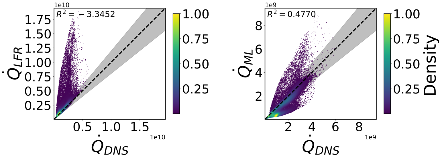
Figure 3 - Parity plots representing the pointwise accuracy of the baseline Laminar Finite Rates model (LFR, on the left) and of the Machine Learning model (ML, on the right).
Spatial distributions of the error and of the predicted correction factor are finally visualized using mid-plane contour plots.
gamma_2D = gamma.reshape(filtered_field.shape)[:,:,filtered_field.shape[2]//2] # extract the z midplane of gamma
HRR_LFR_2D = HRR_LFR.reshape(filtered_field.shape)[:,:,filtered_field.shape[2]//2]# extract the z midplane
HRR_ML_2D = gamma_2D * HRR_LFR_2D
HRR_DNS_2D = HRR_DNS.reshape(filtered_field.shape)[:,:,filtered_field.shape[2]//2]# extract the z midplane

f = ap.contour_plot(filtered_field.mesh.X_midZ*1000,   # Extract x mesh on the z midplane
                  filtered_field.mesh.Y_midZ*1000,   # Extract y mesh on the z midplane
                  np.abs(HRR_LFR_2D-HRR_DNS_2D),
                  vmax=1.5e10,
                  colormap='Reds',
                  x_name='x [mm]',
                  y_name='y [mm]',
                  title=r'$|\dot{Q}_{LFR}-\dot{Q}_{DNS}|$'
                  )

f = ap.contour_plot(filtered_field.mesh.X_midZ*1000,   # Extract x mesh on the z midplane
                  filtered_field.mesh.Y_midZ*1000,   # Extract y mesh on the z midplane
                  np.abs(HRR_ML_2D-HRR_DNS_2D),
                  vmax=1.5e10,
                  colormap='Reds',
                  x_name='x [mm]',
                  y_name='y [mm]',
                  title=r'$|\dot{Q}_{ML}-\dot{Q}_{DNS}|$'
                  )

# Visualize the NN output
f = ap.contour_plot(filtered_field.mesh.X_midZ*1000,   # Extract x mesh on the z midplane
                  filtered_field.mesh.Y_midZ*1000,   # Extract y mesh on the z midplane
                  gamma_2D,
                  colormap='viridis',
                  x_name='x [mm]',
                  y_name='y [mm]',
                  title=r'$\gamma_{NN}$'
                  )
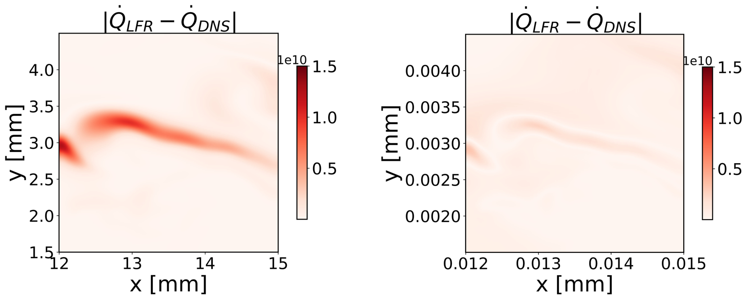
Figure 4 - Absolute error of the baseline physics-based model LFR (left) on the xy physical space; absolute error of the machine learning model (right), typo on the figure title (\(\dot{Q}_{LFR} -> \dot{Q}_{ML}\))
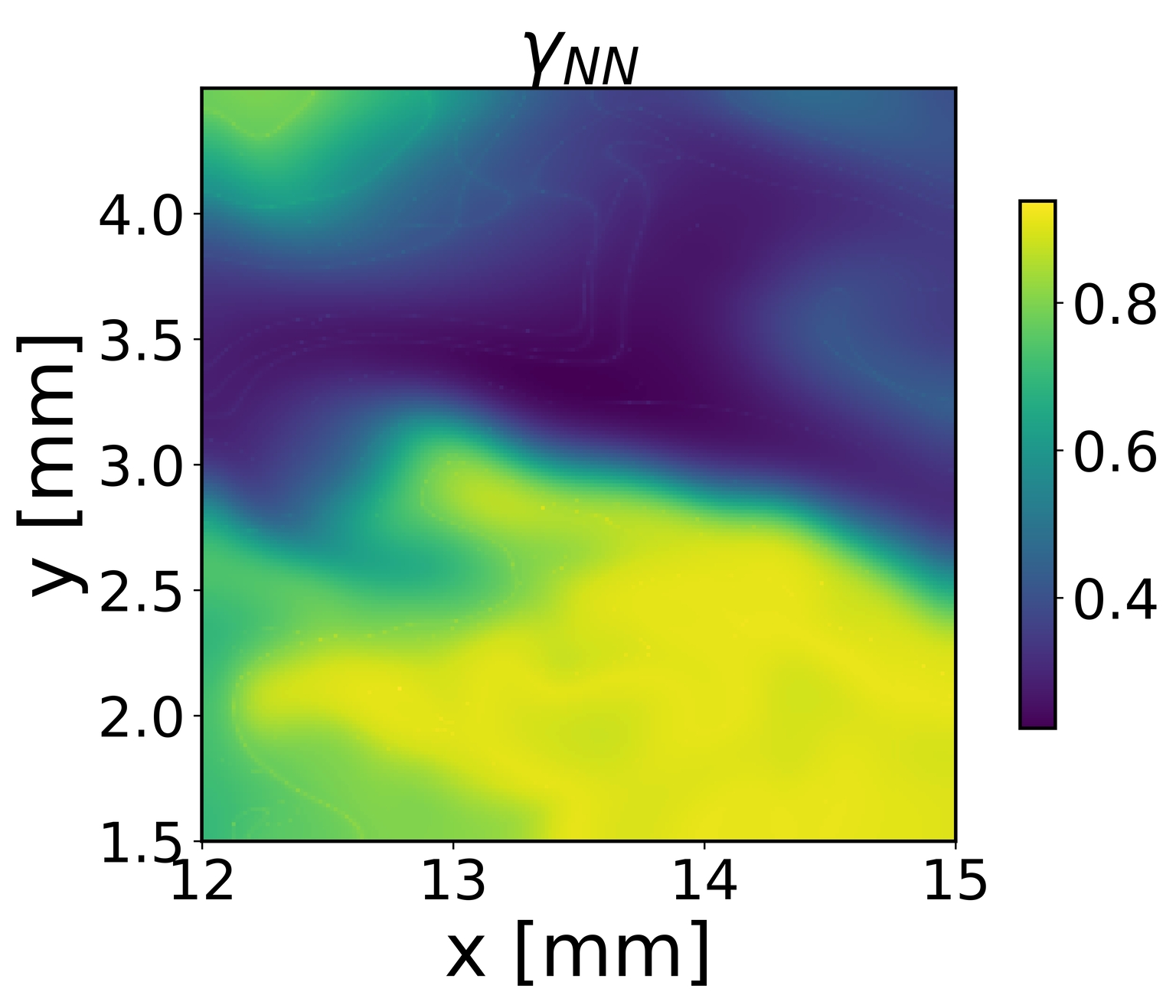
Figure 5 - Plot in the physical space of the cell reacting fraction computed with the machine learning model.