Quickstart
The following tutorial is intended for users who want a quick introduction to basic operations with the library. For a more thorough understanding and detailed explanations, please refer to the comprehensive tutorials available in the Fundamentals and usage section.
This section assumes you have already installed the library. If you haven’t installed it yet, please refer to the Installation page for instructions.
Optional: run tutorial with a different dataset
To follow this hands-on quickstart, you have two options:
Use a dataset from BlastNet
You can select any case that provides data for a single timestep (the current version of the library assumes one time index per dataset). Download the case locally and point
aPriorito the top-level folder of the dataset.Use the reduced example dataset on GitHub
A small example dataset, extracted from a slot-burner hydrogen flame simulation, is available in the project repository. This dataset is formatted to be immediately compatible with
aPrioriand is convenient if you just want to test the library without browsing external databases.You can either download it manually from the GitHub repo or use the convenience helper provided by the package (see the tutorials for a complete example).
First step: download hydrogen diffusion flame DNS
As a first step we are going to download the dataset. Figure 1 shows a representation of the subdomain used in this tutorial.
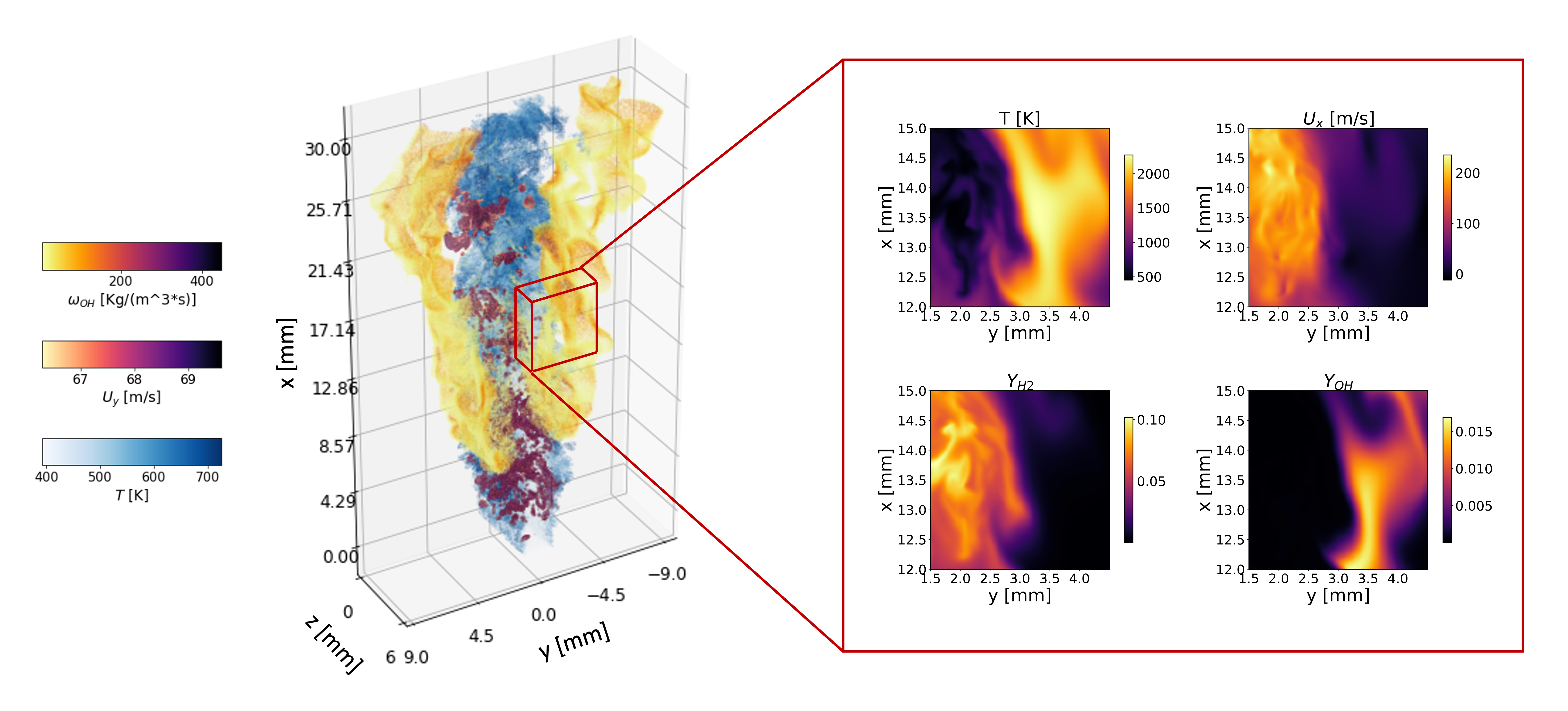
Figure 1: Graphical representation of the DNS subset used in the present tutorial
Run the following command to download the dataset:
import aPriori as ap

ap.download(dataset='h2_lifted')
This command should have downloaded from Github a folder with the following structure:
Lifted_H2_subdomain/
├── chem_thermo_tran/
│   ├── li_h2.cti
│   └── li_h2.yaml
├── data/
│   ├── P_Pa_id000.dat
│   ├── RHO_kgm-3_id000.dat
│   ├── T_K_id000.dat
│   ├── UX_ms-1_id000.dat
│   ├── UY_ms-1_id000.dat
│   ├── UZ_ms-1_id000.dat
│   ├── YH2_id000.dat
│   ├── YH2O_id000.dat
│   ├── YH_id000.dat
│   ├── YN2_id000.dat
│   ├── YNO_id000.dat
│   ├── YO2_id000.dat
│   ├── YOH_id000.dat
│   └── Z_id000.dat
├── grid/
│   ├── X_m.dat
│   ├── Y_m.dat
│   └── Z_m.dat
└── info.json
Visualization
After downloading the dataset, the following lines of code initialize a Field3D object. Once instantiated the object, we can display the field leveraging the plotting utilities:
# Initialize 3D DNS field
field_DNS = ap.Field3D('Lifted_H2_subdomain')

#----------------------------Visualize the dataset-----------------------------#

# Plot Temperature on the xy midplane (transposed as yx plane)
field_DNS.plot_z_midplane('T',                 # plots the Temperature
                        levels=[1400, 2000], # isocontours at 1400 and 2000
                        vmin=1400,           # minimum temperature to plot
                        title='T [K]',       # figure title
                        linewidth=2,         # isocontour lines thickness
                        transpose=True,      # inverts x and y axes
                        x_name='y [mm]',     # x axis label
                        y_name='x [mm]')     # y axis label
# Plot Temperature on the xz midplane (transposed as zx plane)
field_DNS.plot_y_midplane('T',
                        levels=[1400, 2000],
                        vmin=1400,
                        title='T [K]',
                        linewidth=2,
                        transpose=True,
                        x_name='z [mm]',
                        y_name='x [mm]')
# Plot Temperature on the yz midplane
field_DNS.plot_x_midplane('T', levels=[1400, 2000], vmin=1400,
                        title='T [K]', linewidth=2)
# Plot OH mass fraction on the transposed xy midplane
field_DNS.plot_z_midplane('YOH', title=r'$Y_{OH}$', colormap='inferno',
                        transpose=True, x_name='z [mm]', y_name='x [mm]')
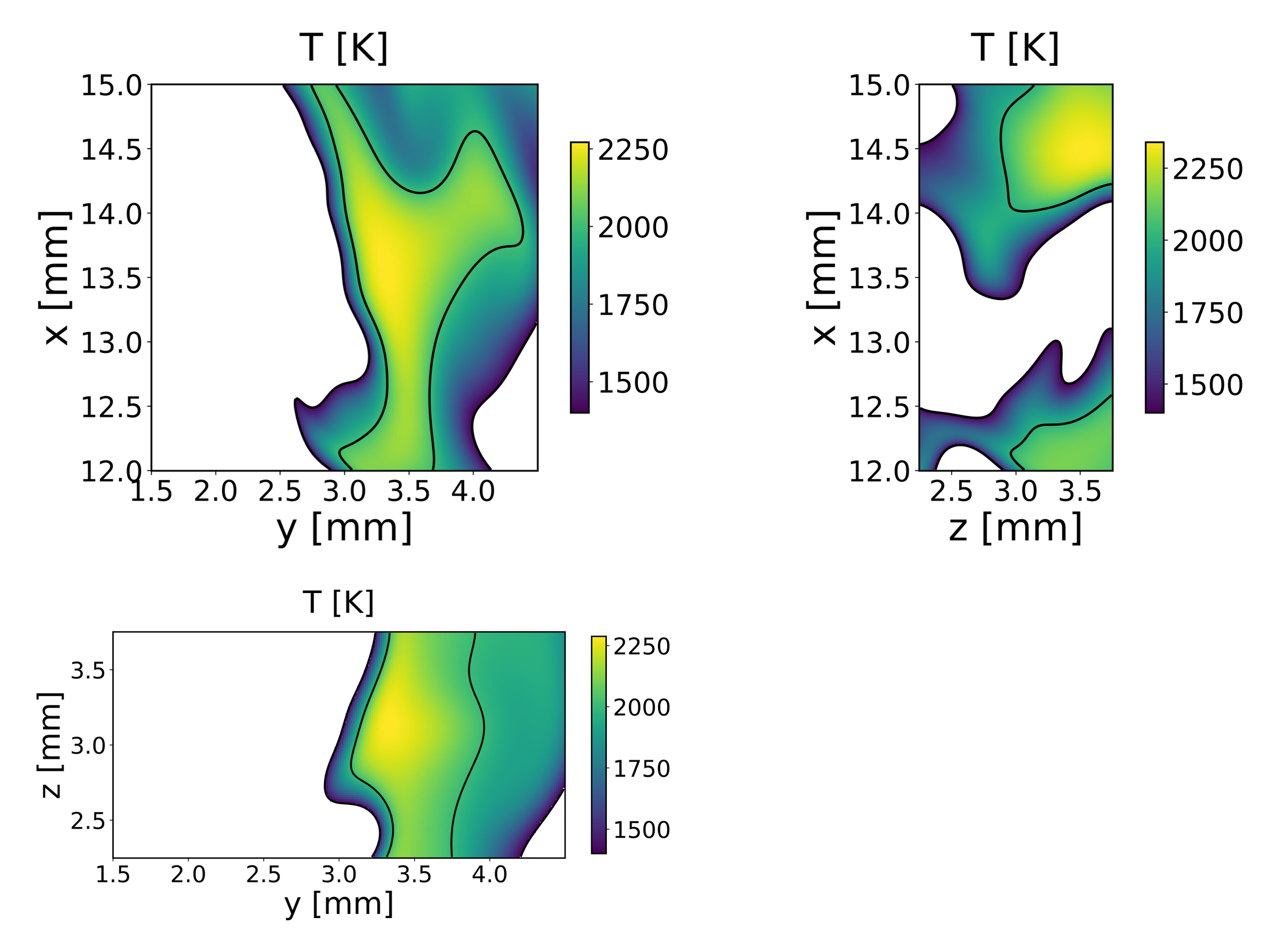
Figure 2 - Temperature field on the x, y, and z midplanes.
Compute reaction rates on DNS field
The reaction rates are computed using Cantera.
The method compute_reaction_rates() uses data chunking to allow large files to be read without causing memory issues. The optional input parameter n_chunks defines in how many chunks the files to be read and to be written are divided.
To compute the instantaneous rates the values of temperature, pressure, and species concentration are necessary. The chemical mechanism in the chem_thermo_tran directory is used to compute the rates in every cell.
After the computation, new files in the folder ‘data/’ will be saved to store the reaction rates, for example, the hydrogen reaction rate will be named ‘RH2_DNS_kgm-3s-1_id000.dat’. The suffix DNS is used to distinguish the rates computed on the unfiltered grid to the ones computed on the filtered grid (that will be shown later on in the tutorial).
#--------------------------Compute DNS reaction rates--------------------------
field_DNS.compute_reaction_rates()
# Plot OH mass fraction on the transposed xy midplane
field_DNS.plot_z_midplane('YOH', title=r'$Y_{OH}$ $[-]$', colormap='inferno',
transpose=True, x_name='z [mm]', y_name='x [mm]')
# Plot reaction rates
field_DNS.plot_z_midplane('ROH_DNS',
title=r'$\dot{\omega}_{OH}$ $[kg/m^3/s]$',
colormap='inferno',
transpose=True, x_name='z [mm]', y_name='x [mm]')
field_DNS.plot_z_midplane('RH2O_DNS',
title=r'$\dot{\omega}_{H2O}$ $[kg/m^3/s]$',
colormap='inferno',
transpose=True, x_name='z [mm]', y_name='x [mm]')
#--------------------------Compute derived variables---------------------------
# compute kinetic energy
field_DNS.compute_kinetic_energy()
# Compute mixture fraction
field_DNS.ox = 'O2' # Defines the species to consider as oxydizer
field_DNS.fuel = 'H2' # Defines the species to consider as fuel
Y_ox_2=0.233 # Oxygen mass fraction in the oxydizer stream (air)
Y_f_1=0.65*2/(0.65*2+0.35*28) # Hydrogen mass fraction in the fuel stream
# (the fuel stream is composed by X_H2=0.65 and X_N2=0.35)
field_DNS.compute_mixture_fraction(Y_ox_2=Y_ox_2, Y_f_1=Y_f_1, s=2)
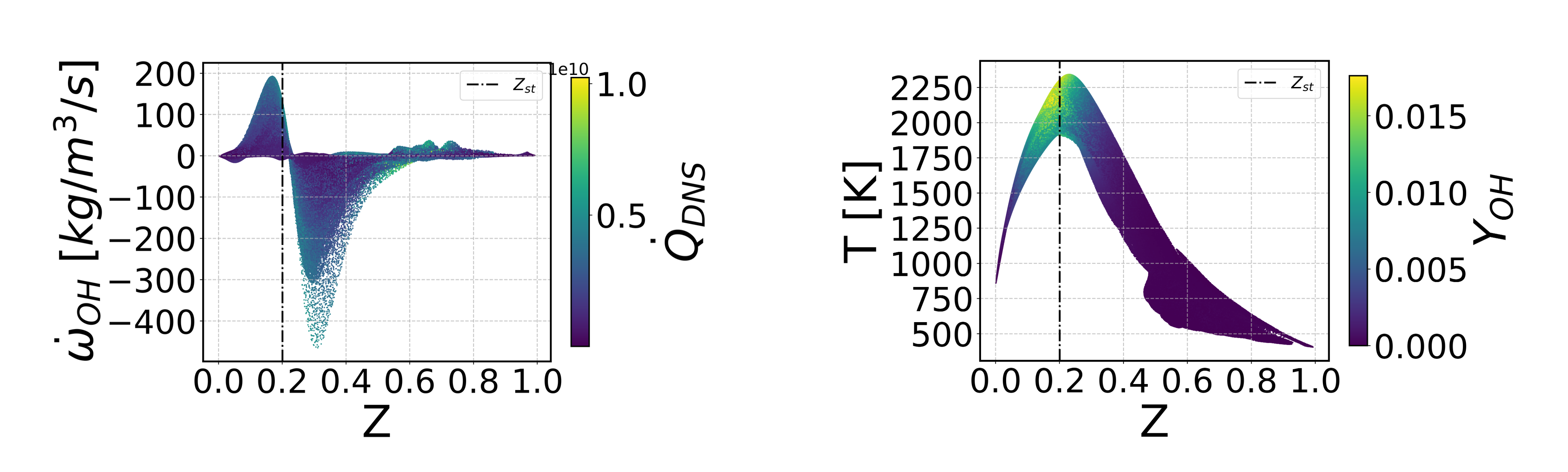
# Scatter plot variables as functions of the mixture fraction Z
field_DNS.scatter_Z('T', # the variable to plot on the y axis
c=field_DNS.YOH.value, # set color of the points
y_name='T [K]',
cbar_title=r'$Y_{OH}$'
)
field_DNS.scatter_Z('ROH_DNS',
c=field_DNS.HRR_DNS.value,
y_name=r'$\dot{\omega}_{OH}$ $[kg/m^3/s]$',
cbar_title=r'$\dot{Q}_{DNS}$'
)

Filtering
The object’s filtering function will create a secondary folder, with the same structure as the main folder containing the unfiltered data. The function returns a string with the folder name, that in this case is “Filter16FavreGauss”. The filter size, the filter kernel (Box, Gaussian, etc…) are included in the folder name to define the filtering operation that was used to obtain the dataset. The word “Favre” appears in the folder’s name if Favre filtering was used.
All the files contained in the data folder when the command is launched will be automatically filtered by the filtering function.
#-------------------------------Filter DNS field-------------------------------
# perform favre filtering (high density gradients)
# the output of the function is a string with the new folder's name, f_string
f_string = field_DNS.filter_favre(filter_size=16, # filter amplitude
                                       filter_type='Gauss') # 'Gauss' or 'Box'

# The string with the folder's name is now used to initialize the filered field
field_filtered = ap.Field3D(f_string)

# Visualize the effect of filtering on the Heat Release Rate
field_DNS.plot_z_midplane('HRR_DNS',
                        title=r'$\dot{Q}_{DNS}$ $[W/m^3]$',
                        colormap='inferno',
                        vmax=8*1e9,
                        transpose=True, x_name='z [mm]', y_name='x [mm]',
                        remove_cbar=True)

field_filtered.plot_z_midplane('HRR_DNS',
                        title=r'$\overline{\dot{Q}_{DNS}}$ $[W/m^3]$',
                        colormap='inferno',
                        vmax=8*1e9,
                        transpose=True, x_name='z [mm]', y_name='x [mm]',
                        remove_y=True)
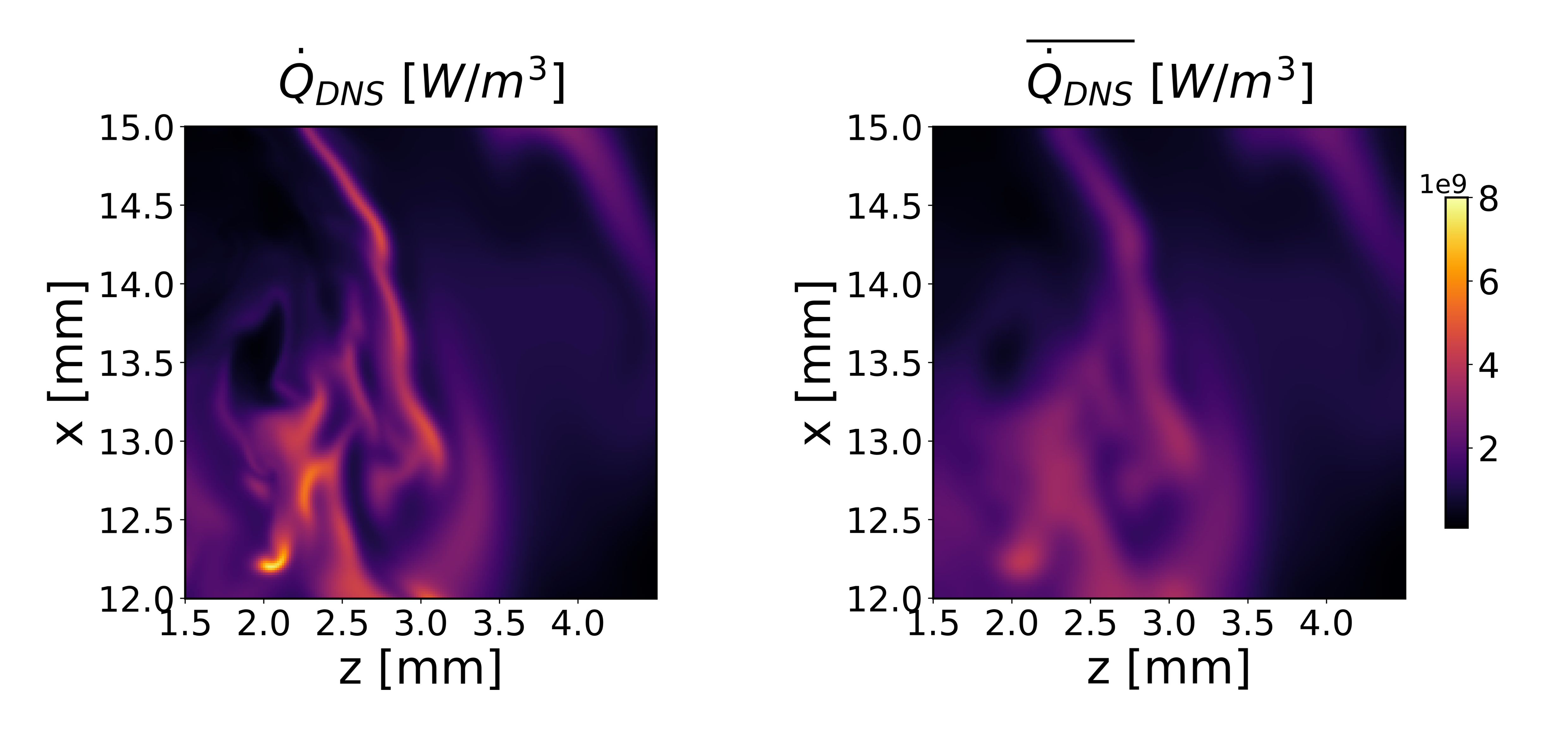
Figure 5 - Original vs filtered heat release rates
Compute laminar rates on the filtered field
The filtered field is what in a priori validation is considered to resemble a Large Eddy Simulation (LES) snapshot. From those values, it is possible to model the unclosed quantities, and then compare them with the DNS benchmark values.
The simplest way to model the reaction rates is based on the so-called Laminar Finite Rate (LFR) approximation. This approach directly computes the reaction rates from the filtered LES field:
Where:
\(\bar{\dot{\omega}}_{\mathrm{LFR}}\) represents the reaction rates.
\(\dot{\omega}(\tilde{T}, \tilde{Y}_k)\) is the computation of the instantaneous Arrhenius rates from the filtered temperature \(\tilde{T}\) and the filtered species concentrations \(\tilde{Y}_k\).
This code snippet computes \(\bar{\dot{\omega}}_{\mathrm{LFR}}\) and compares it with the filtered DNS values \(\bar{\dot{\omega}}_{\mathrm{DNS}}\). For more complex modeling approaches, see the section Machine Learning Tutorials at the paragraph Data-Driven Closure for Turbulence–Chemistry Interaction.
#-------------------------Compute reaction rates (LFR)-------------------------
# Computing reaction rates directly from the filtered field (LFR approximation)
field_filtered.compute_reaction_rates()

# Compare visually the results
field_filtered.plot_z_midplane('RH2_DNS',
                        title=r'$\overline{\dot{\omega}}_{H2}^{DNS}$ $[kg/(m^3\cdot s)]$',
                        vmax=-20,
                        vmin=field_filtered.RH2_LFR.z_midplane.min(),
                        levels=[-300, -50, -20],
                        labels=True,
                        colormap='inferno',
                        transpose=True, x_name='z [mm]', y_name='x [mm]',
                        remove_cbar=True)

# Compare visually the results in the z midplane
field_filtered.plot_z_midplane('RH2_LFR',
                        title=r'$\overline{\dot{\omega}}_{H2}^{LFR}$ $[kg/(m^3\cdot s)]$',
                        vmax=-20,
                        vmin=field_filtered.RH2_LFR.z_midplane.min(),
                        levels=[-300, -50, -20],
                        labels=True,
                        colormap='inferno',
                        transpose=True, x_name='z [mm]', y_name='x [mm]',
                        remove_y=True)

# Compare the heat release rate results with a parity plot
f = ap.parity_plot(field_filtered.HRR_DNS.value,  # x
                  field_filtered.HRR_LFR.value,  # y
                  density=True,                  # KDE coloured
                  x_name=r'$\overline{\dot{\omega}}_{H2}^{DNS}$',
                  y_name=r'$\overline{\dot{\omega}}_{H2}^{LFR}$',
                  cmin=0,
                  RMSE=False,
                  NRMSE=True,
                  ticks=[0, 0.8e10, 1.6e10]
                  )
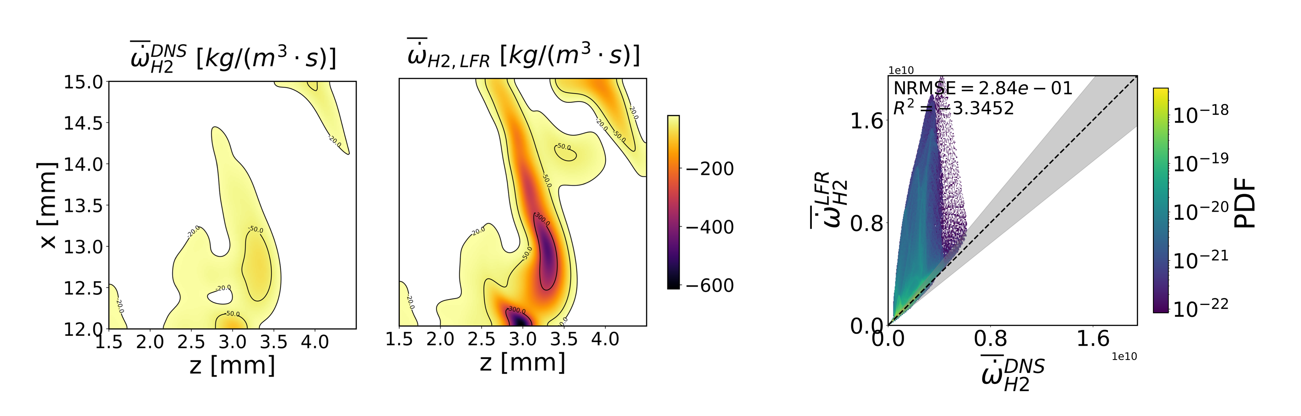
Figure 6 - Filtered hydrogen reaction rate computed on the original grid (DNS), hydrogen laminar finite rates (LFR) computed on the filtered grid, parity plot comparing the two results.