Tutorial 8: Computational Singular Perturbation (CSP) analysis

Note

The complete code associated with this tutorial is available here.

This tutorial demonstrates how to perform Computational Singular Perturbation (CSP) analysis on DNS data using the coupling between the aPriori and PyCSP packages.

CSP analysis provides diagnostic tools to understand the chemical dynamics in reacting flows by decomposing the system into fast and slow modes. Two key quantities available in this implementation are:

• Tangential Stretching Rate (TSR): identifies the characteristic chemical time scale and distinguishes between explosive (TSR > 0) and dissipative (TSR < 0) regions in the flow field.

• Amplitude Participation Indexes (APIs): quantify which chemical reactions or transport processes contribute most to the dynamics of each mode, enabling detailed cause-effect analysis.

The TSR is particularly useful for identifying where fast chemistry dominates and for defining local Damköhler numbers. APIs help pinpoint which specific reactions control ignition, flame propagation, or radical production.

For detailed theoretical background on CSP, TSR, and APIs, and usage of PyCSP see Valorani et al. [24] and Malpica Galassi. [25]

Import modules and define data path

Imports and paths definition

import os
import aPriori as ap
from aPriori import DNS

# Download the example dataset
ap.download(dataset='csp')

# Define path to the DNS data folder
directory = os.path.join('.', 'Lifted_H2_subdomain_csp')
figures_folder = 'figures_csp'

# Check if data exists
if not os.path.exists(directory):
    print("Dataset not found. Downloading from Github...")
    ap.download(dataset='csp')

Compute CSP quantities

The compute_csp() method performs the full CSP decomposition on the 3D field, computing eigenvalues, eigenvectors, modal amplitudes, and participation indices. The API_species parameter allows you to select which species to analyze in detail. Processing automatically uses data-chunking to handle large datasets efficiently.

Loading the field and computing CSP quantities

# Load the DNS field
dns_field = ap.Field(directory)

# Compute CSP quantities (TSR and APIs)
# Specify species for which to compute APIs
dns_field.compute_csp(
    API_species=['H2O', 'OH'],
    n_chunks=100,  # Number of chunks for parallel processing
)

# Create output directory
os.makedirs(figures_folder, exist_ok=True)

Visualize TSR-based participation indices

This visualization shows which chemical reactions have the largest influence on the system’s dynamics. Reactions with positive participation (red) accelerate the dynamics, while those with negative participation (gray) have a damping effect. The dynamics can be locally either dissipative or explosive, depending on the TSR, which will be visualized in Fig. 3.

Plot reactions contributing to the TSR

# Plot the top 10 reactions contributing to TSR
dns_field.plot_api(
    api_type='TSR',
    n=10,           # Number of top reactions to display
    n_cols=5,       # Layout: 2 rows, 5 columns
    cmap='RdGy_r',  # Diverging colormap
    vmin=-1, vmax=1,
    save_path=os.path.join(figures_folder, 'api_tsr.png')
)

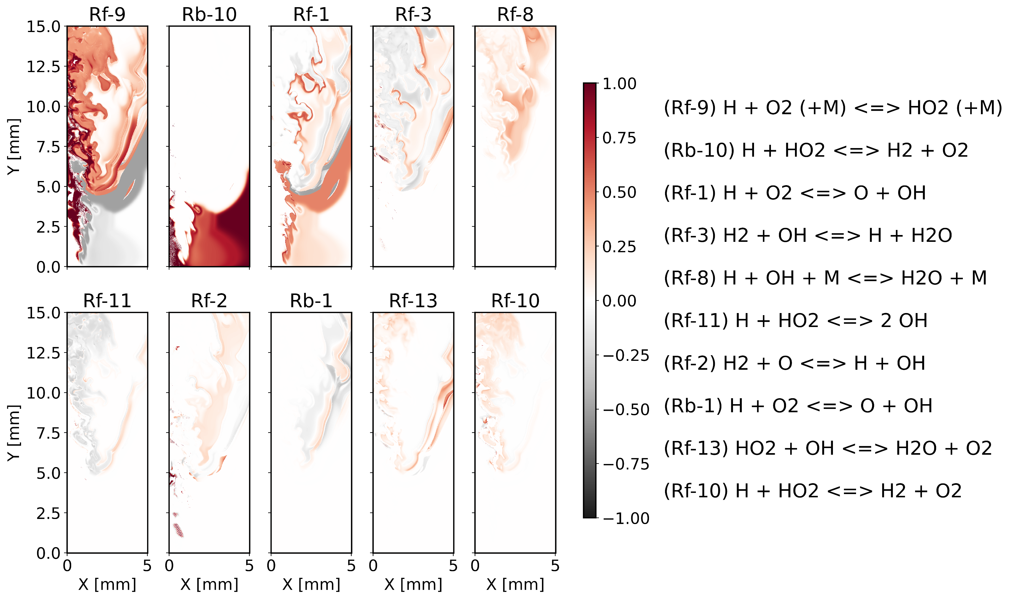
Figure 1 - TSR-based amplitude participation indices for the 10 most important reactions. Chain-branching reactions like H + O₂ ⇌ O + OH dominate in explosive regions, while termination steps appear in dissipative zones.

Visualize species-specific participation indices

Species-specific APIs reveal which reactions produce or consume a particular species. This is useful for understanding pollutant formation pathways or radical production mechanisms. The spatial distribution shows where each reaction is most active in controlling that species.

Plot reactions affecting OH production

# Plot reactions controlling OH chemistry
dns_field.plot_api(
    api_type='OH',  # Species-specific APIs
    n=10,
    n_cols=5,
    cmap='RdGy_r',
    vmin=-1, vmax=1,
    save_path=os.path.join(figures_folder, 'api_oh.png')
)

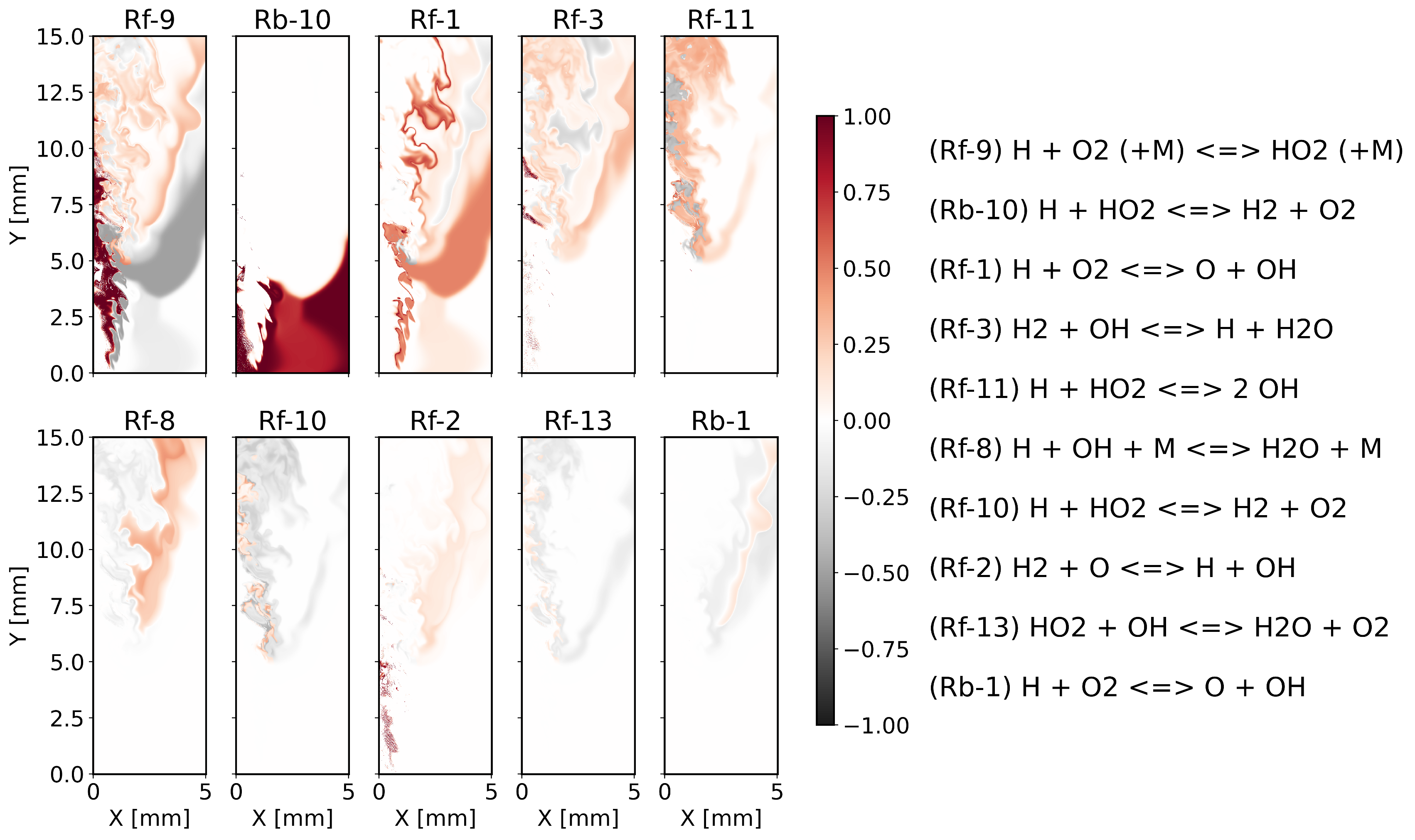
Figure 2 - OH-based amplitude participation indices for the 10 most important reactions. These indices reveal which reactions directly produce or consume OH radicals. The spatial patterns are more localized than TSR-based APIs, closely following the thin reaction layer where OH chemistry is most active. Reactions like H₂ + OH ⇌ H + H₂O show strong participation in the flame zone, while chain-branching steps remain important for radical production.

Plot TSR spatial distribution

Separating positive and negative TSR values helps identify different chemical regimes. Positive TSR indicates explosive chain-branching chemistry, typically concentrated at the flame front. Negative TSR corresponds to dissipative relaxation toward chemical equilibrium.

Visualize TSR field on midplane

# Plot negative TSR values (dissipative regions)
dns_field.plot_z_midplane(
    'TSR_DNS',
    colormap='gist_heat',
    transpose=True,
    remove_title=True,
    cbar_title='TSR $[s^{-1}]$',
    vmax=0,  # Show only negative values
    transparent=False,
    save_path=os.path.join(figures_folder, 'TSR_negative.png')
)

# Plot positive TSR values (explosive regions)
dns_field.plot_z_midplane(
    'TSR_DNS',
    colormap='gist_heat_r',
    transpose=True,
    remove_title=True,
    cbar_title='TSR $[s^{-1}]$',
    vmin=0,  # Show only positive values
    transparent=False,
    remove_y=True,
    save_path=os.path.join(figures_folder, 'TSR_positive.png')
)

Figure 3 - Spatial distribution of TSR: (left) negative values showing dissipative regions, (right) positive values revealing explosive chemistry localized at the flame front.

Compare with physical fields

Comparing CSP diagnostics with traditional physical fields (temperature, species mass fractions) provides validation and physical insight. Regions of high TSR magnitude typically coincide with peaks in radical concentrations and heat release, confirming the coupling between fast chemistry and flame structure.

Plot OH mass fraction and temperature

# Plot OH mass fraction
dns_field.plot_z_midplane(
    'YOH',
    colormap='gist_heat_r',
    transpose=True,
    remove_title=True,
    cbar_title=r'$Y_{OH}$ $[-]$',
    save_path=os.path.join(figures_folder, 'YOH.png')
)

# Plot temperature field
dns_field.plot_z_midplane(
    'T',
    colormap='gist_heat_r',
    transpose=True,
    remove_title=True,
    remove_y=True,
    cbar_title=r'$T$ $[K]$',
    save_path=os.path.join(figures_folder, 'T.png')
)

Figure 4 - Physical fields for comparison: (left) OH mass fraction marking the reaction zone, (right) temperature field showing heat release regions.

Key takeaways

This tutorial demonstrates how CSP analysis in aPriori enables:

1. Time scale identification: TSR quantifies the fastest chemical time scale and separates explosive from dissipative regions.

2. Reaction pathway analysis: APIs reveal which specific reactions control the system dynamics or individual species evolution.

3. Spatial diagnostics: All CSP quantities can be visualized on the DNS mesh, enabling detailed spatial analysis of chemical regimes.

These tools are particularly valuable for:

• Analyzing ignition and extinction events

• Identifying rate-limiting steps in complex mechanisms

• Understanding pollutant formation pathways

• Guiding mechanism reduction strategies

• Validating reduced-order models

For advanced applications, CSP outputs can be combined with other aPriori features such as filtered fields or conditional statistics to study the interaction between turbulence and chemistry at multiple scales.