Tutorial 4: Data visualization

Note

The complete code associated with this tutorial is available here.

This exercise introduces some of the main data-visualization utilities provided by the library. These tools are designed for rapid inspection of DNS fields and for the generation of publication-quality, single-figure plots with minimal user input.

The plotting interface intentionally favors simplicity and consistency over full customizability. As a result, the level of personalization is limited when compared to general-purpose plotting libraries. The current plotting logic is optimized for the creation of individual figures, which can subsequently be combined or arranged during post-processing, rather than for assembling complex figures with multiple subplots within a single call.

Import modules, download dataset, and define data path

Imports and paths definition

import os
import aPriori as ap
import json

# Comment the following line if you already downloaded the dataset
ap.download(dataset='h2_lifted')

# Change this with your path to the data folder if necessary
directory = os.path.join('.','Lifted_H2_subdomain')

# Check the folder with the data exists in your system
T_path = os.path.join(directory,'data', 'T_K_id000.dat')
print(f"\nChecking the path \'{T_path}\' is correct...")
if not os.path.exists(T_path):
   raise ValueError("The path '{T_path}' does not exist in your system. Check to have the correct path to your data folder in the code")
else:
   print("Folder path OK\n")

Initialize field and plot midplanes

Instantiate Field object and plot midplanes

DNS_field = ap.Field(directory)

# Visualize the data
# Default plotting of a variable along the x, y, z midplanes
DNS_field.plot_z_midplane('YH2O2')
DNS_field.plot_y_midplane('YH2O2')
DNS_field.plot_x_midplane('YH2O2')

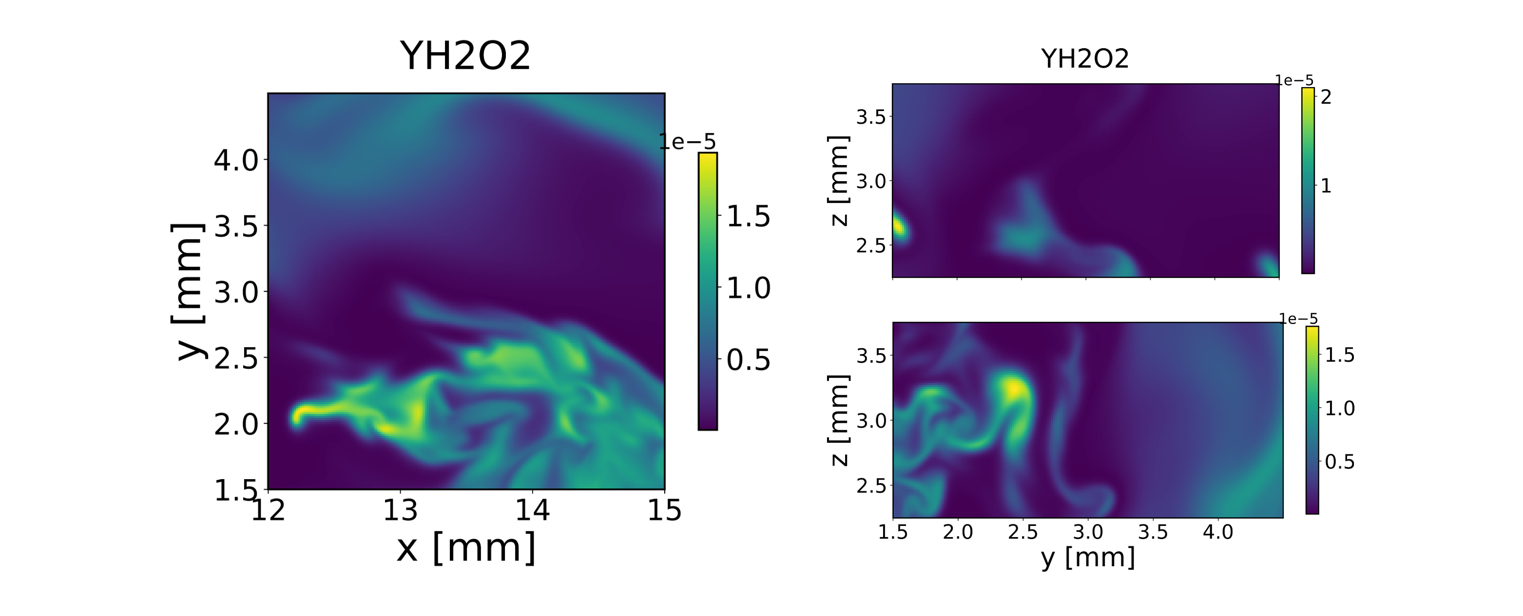
Figure 1 - H2O2 mass fraction field on the x, y, and z midplanes.

The plotting utilities contain various input options to personalize the output. The following code snippet provides an example:

Advanced midplane plots settings

# Advanced settings to plot. We'll consider the z midplane for simplicity
DNS_field.plot_z_midplane('YH2O2',
                        levels=[1e-6,1e-5,1.5e-5], # isocontour lines
                        vmin=1e-6,                 # minimum temperature to plot
                        title=r'$Y_{H2O2}$',       # figure title
                        linewidth=1,               # isocontour lines thickness
                        transpose=True,            # inverts x and y axes
                        x_name='y [mm]',           # x axis label
                        y_name='x [mm]',           # y axis label
                        colormap='inferno_r',        # change colormap
                        )

Figure 2 - H2O2 mass fraction field on the z midplanes, with isolines at 1e-6, 1e-5, and 1.5e-5.

Plots in the mixture fraction space

The mixture fraction \(Z\) represents a conserved scalar that parameterizes the local mixing state between the fuel and oxidizer streams. By construction, \(Z=0\) corresponds to pure oxidizer conditions, while \(Z=1\) corresponds to pure fuel. Intermediate values identify mixed states, independently of chemical reactions.

For reacting flows, many thermochemical quantities (e.g., temperature or species mass fractions) exhibit strong correlations with \(Z\). The scatter representation highlights departures from purely mixing-controlled behavior, which are associated with chemical heat release, differential diffusion effects, or local extinction and reignition. Coloring the scatter points by a reactive marker such as \(Y_{OH}\) helps identify regions of high chemical activity in mixture-fraction space.

Plots in the mixture fraction space

# Scatter variables as functions of the mixture fraction z
# Compute the mixture fraction with the compute_mixture_fraction method
DNS_field.ox = 'O2'     # Defines the species to consider as oxydizer
DNS_field.fuel = 'H2'   # Defines the species to consider as fuel
Y_ox_2=0.233  # Oxygen mass fraction in the oxydizer stream (air)
Y_f_1=0.65*2/(0.65*2+0.35*28) # Hydrogen mass fraction in the fuel stream
# (the fuel stream is composed by X_H2=0.65 and X_N2=0.35)

DNS_field.compute_mixture_fraction(Y_ox_2=Y_ox_2, Y_f_1=Y_f_1, s=2)

# Scatter plot variables as functions of the mixture fraction Z
DNS_field.scatter_Z('T', # the variable to plot on the y axis
                  c=DNS_field.YOH.value, # set color of the points
                  y_name='T [K]',
                  cbar_title=r'$Y_{OH}$'
                  )

DNS_field.scatter_Z('YH2O2', # the variable to plot on the y axis
                  c=DNS_field.YOH.value, # set color of the points
                  y_name=r'$Y_{H2O2}$',
                  cbar_title=r'$Y_{OH}$'
                  )

Figure 3 - Scatter plots of temperature and H2O2 mass fraction in the mixture fraction space.